Fill styles in depth

Every filled geom (geom_sketch_col(), geom_sketch_rect(), geom_sketch_tile(), geom_sketch_polygon(), geom_sketch_ribbon(), geom_sketch_area(), geom_sketch_density(), and the boxplot box) takes a fill_style. Under the hood, all of them are produced by a single Active-Edge-Table scan-line filler (hachure_fill() and friends) that works on arbitrary — including concave — polygons.

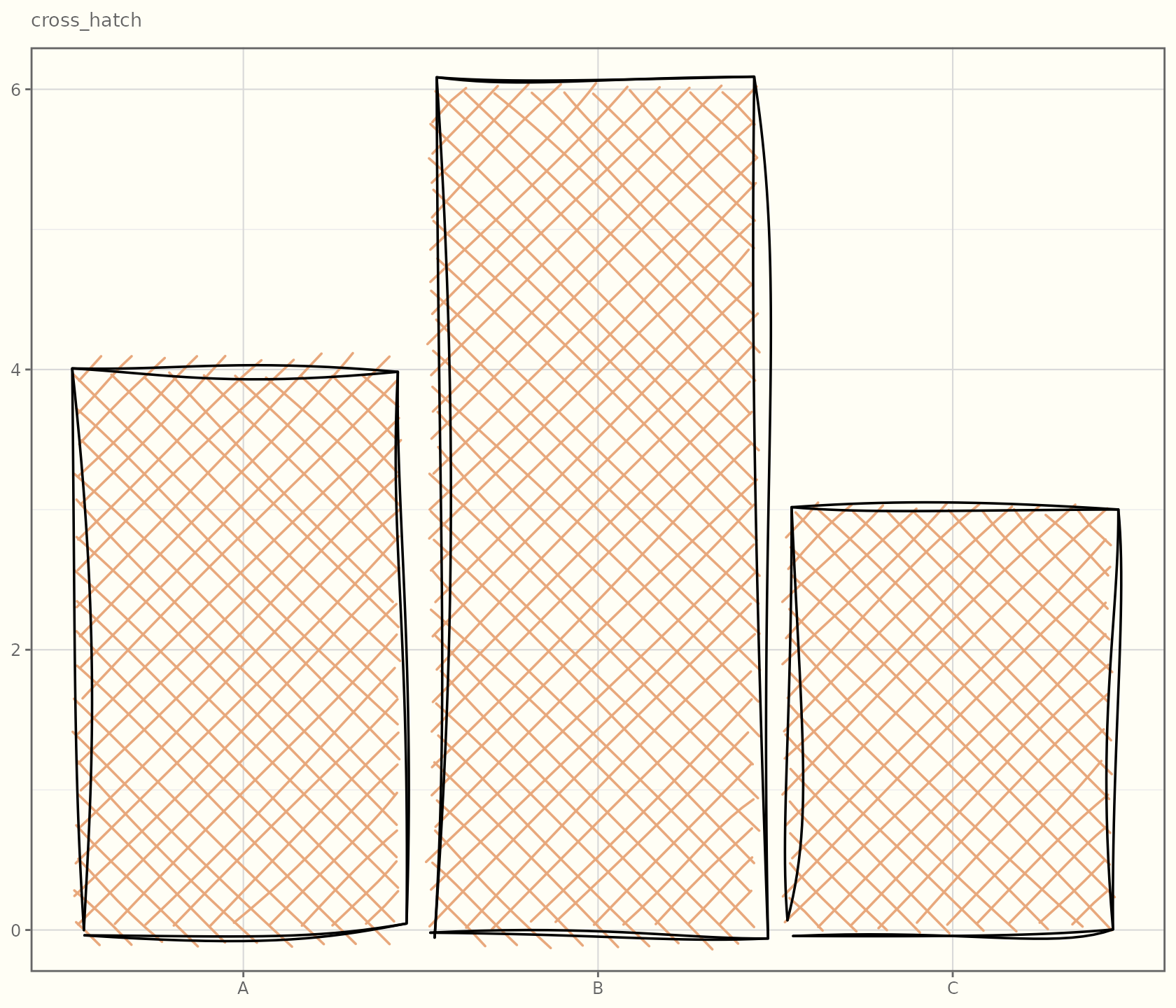
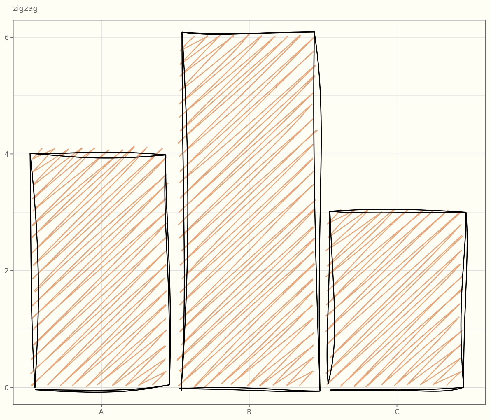
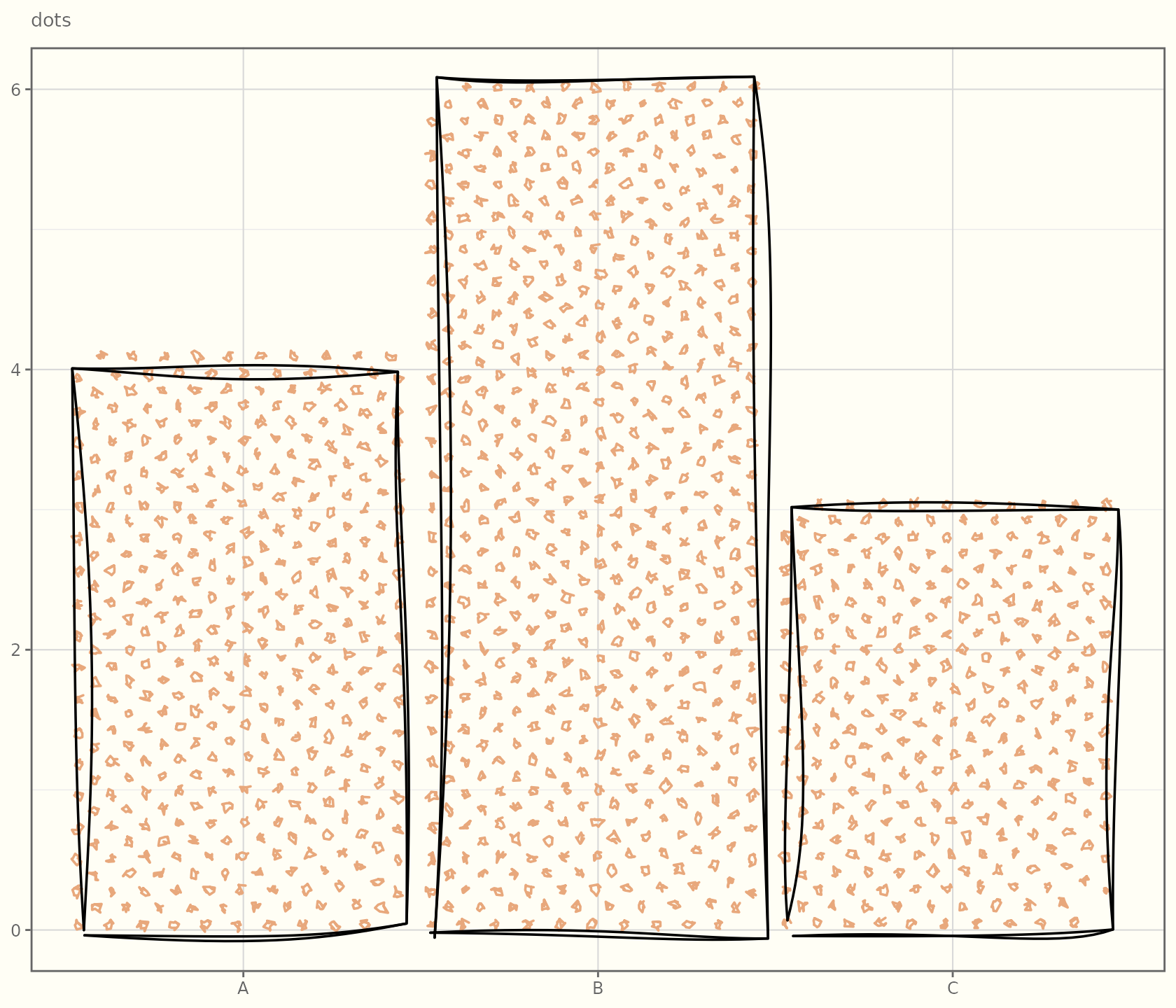
The seven styles

styles <- c("hachure", "cross_hatch", "zigzag", "zigzag_line",
            "dots", "dashed", "solid")

bars <- do.call(rbind, lapply(styles, function(s) {
  data.frame(style = s, x = c("A", "B", "C"), y = c(4, 6, 3))
}))
bars$style <- factor(bars$style, levels = styles)

# Draw a small panel per style by faceting and re-drawing each with its style.
# (fill_style is a layer parameter, so we build one layer per facet.)
plots <- lapply(styles, function(s) {
  ggplot(subset(bars, style == s), aes(x, y)) +
    geom_sketch_col(fill = "#E8A87C", fill_style = s, seed = 4L) +
    labs(subtitle = s, x = NULL, y = NULL) +
    theme_sketch(base_size = 9)
})

# Show them individually:
for (p in plots) print(p)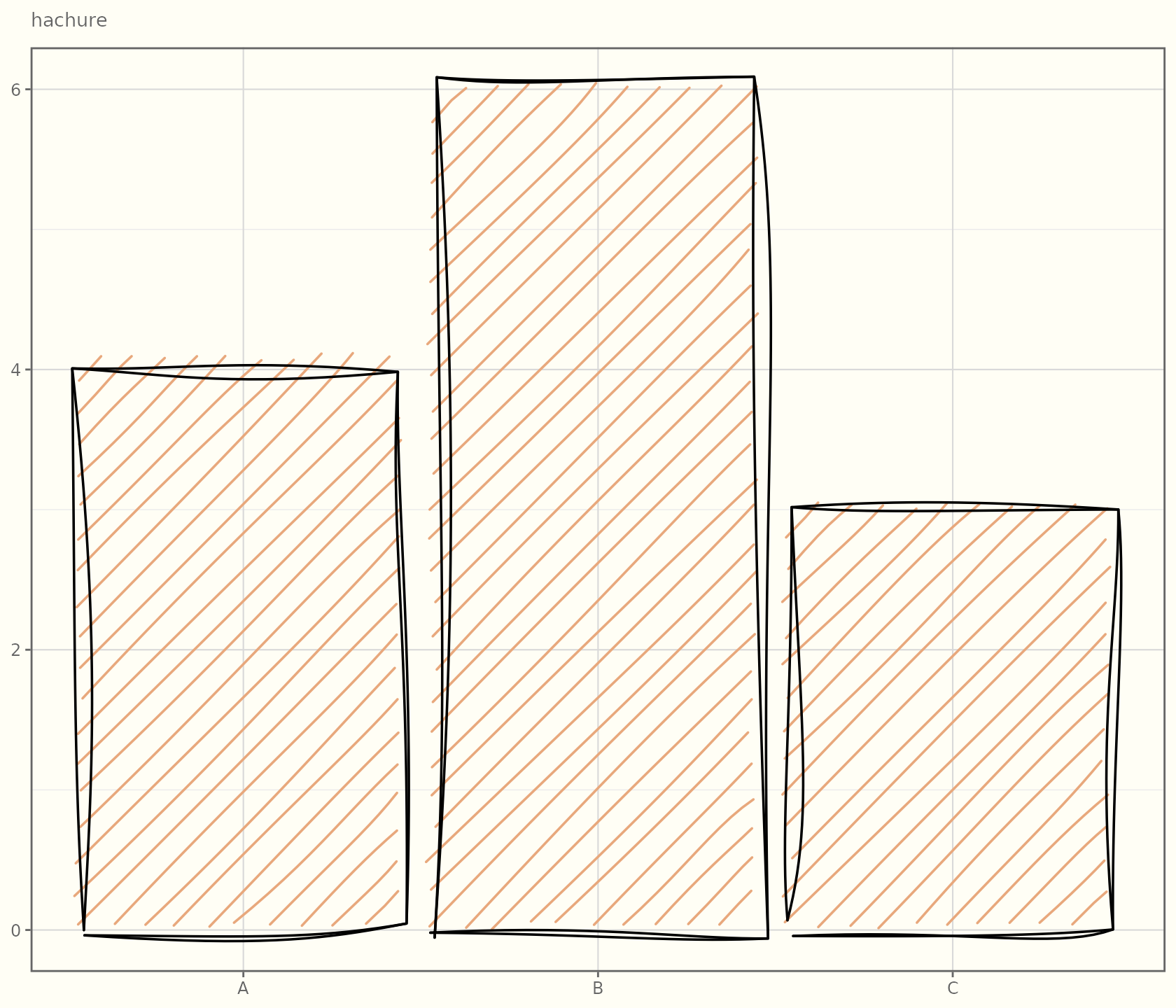

Style	Look	Notes
hachure	Parallel diagonal strokes	The default; classic pencil shading.
cross_hatch	Hachure at angle and angle + 90°	Denser, “darker” shading.
zigzag	Hachure lines joined by diagonal connectors	A continuous scribble feel.
zigzag_line	Just the connectors, as one path	Lighter than zigzag.
dots	Tiny rough circles sampled along the lines	Stippled fill.
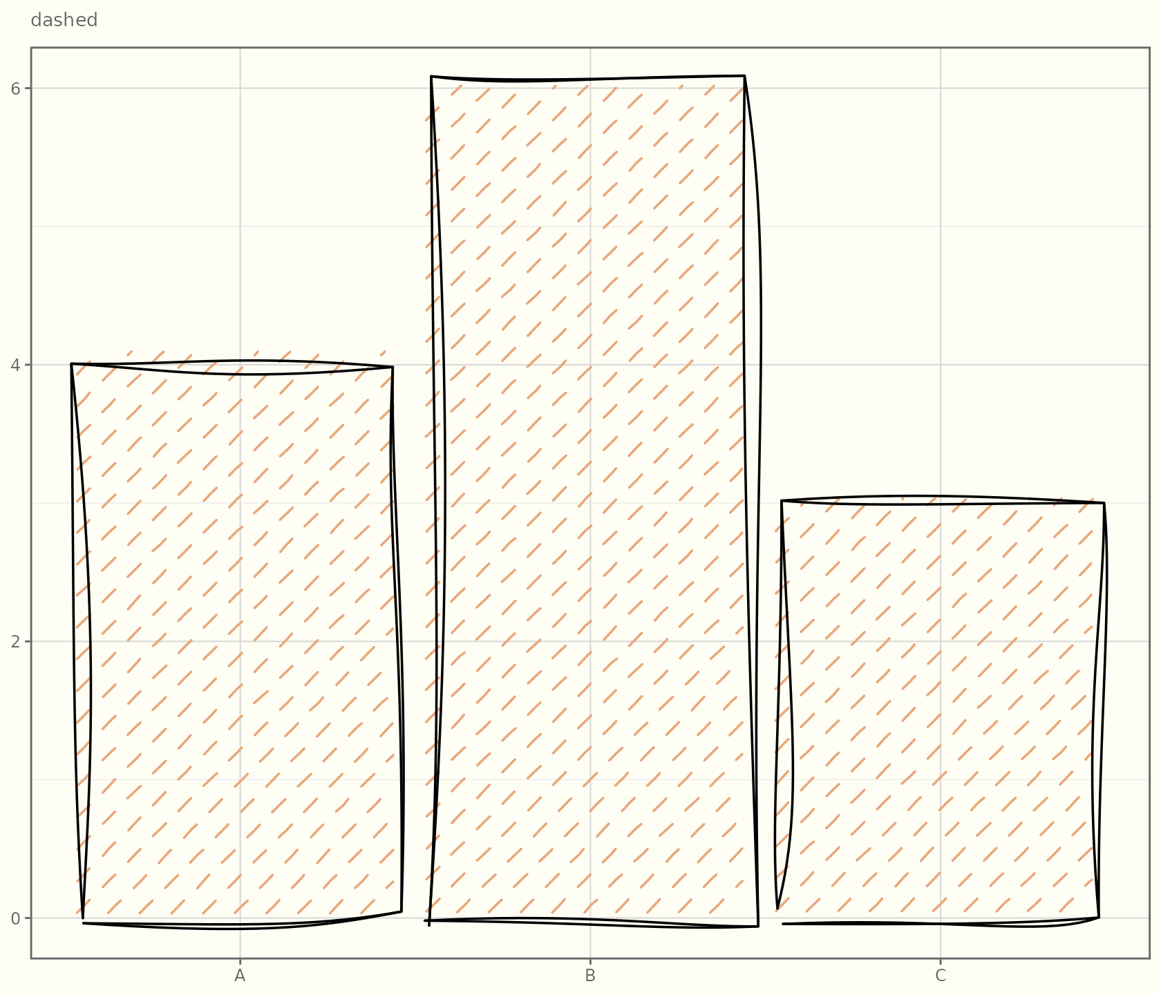
dashed	Hachure broken into dashes	Airy, sketchy texture.
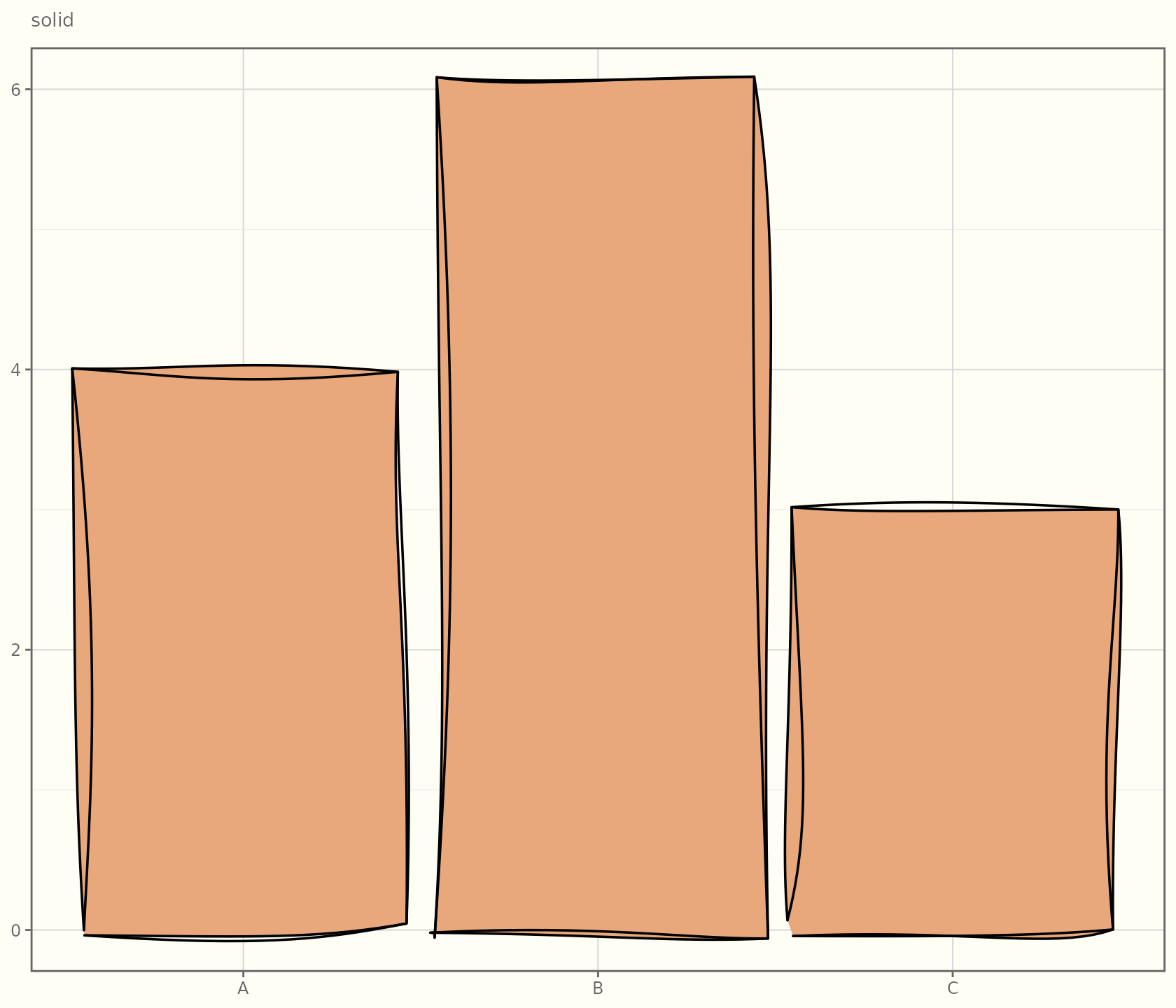
solid	No fill lines (outline only)	Use when you want only the rough outline.

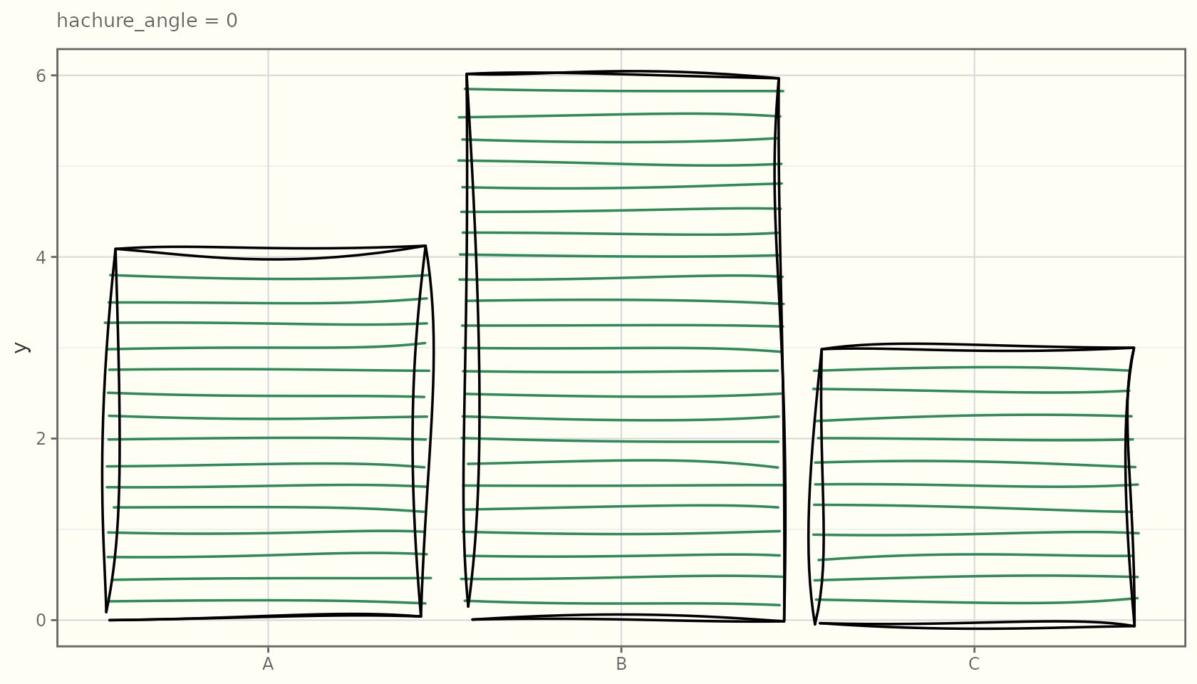
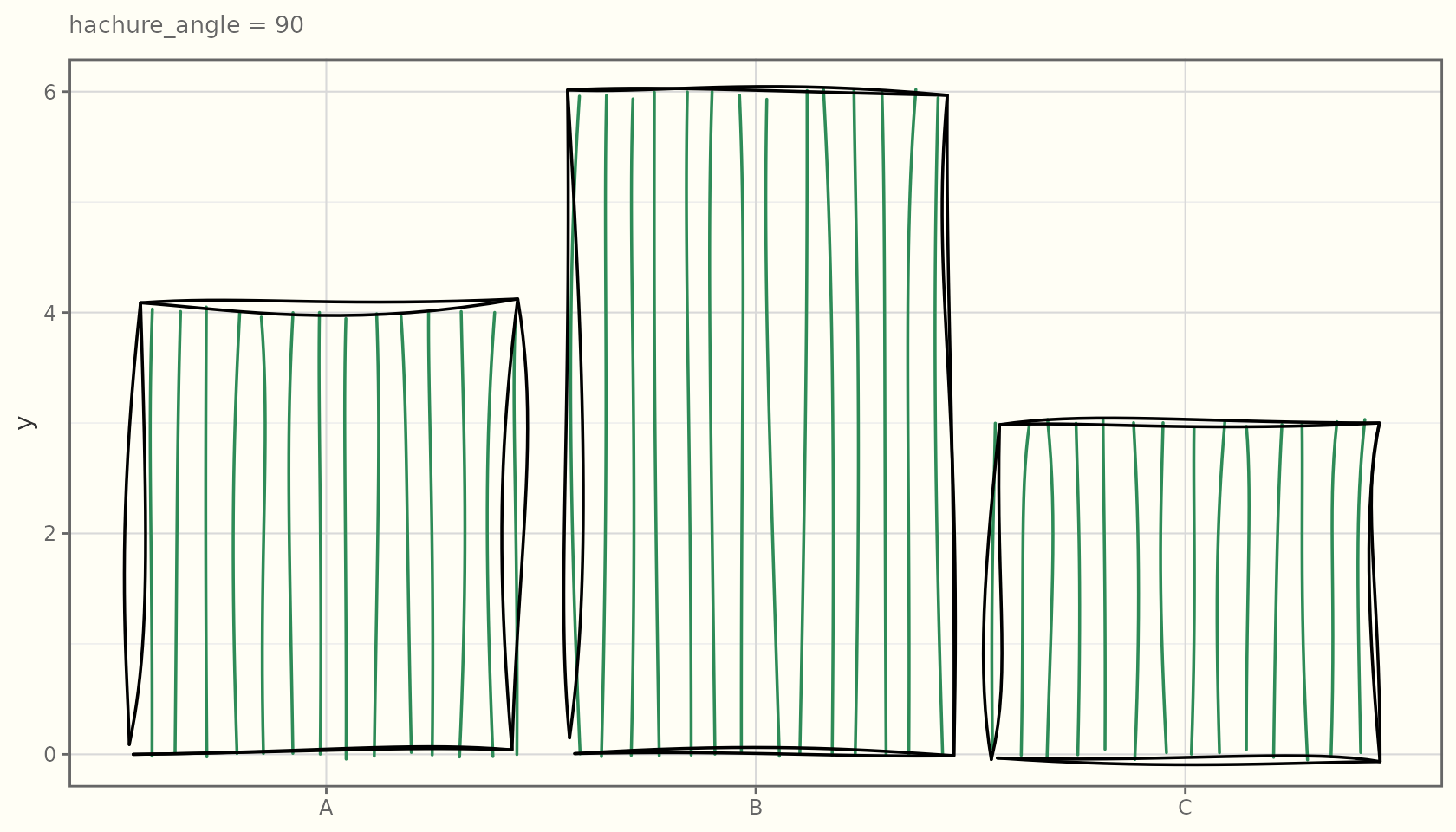
Tuning the hachure

Three parameters control the texture.

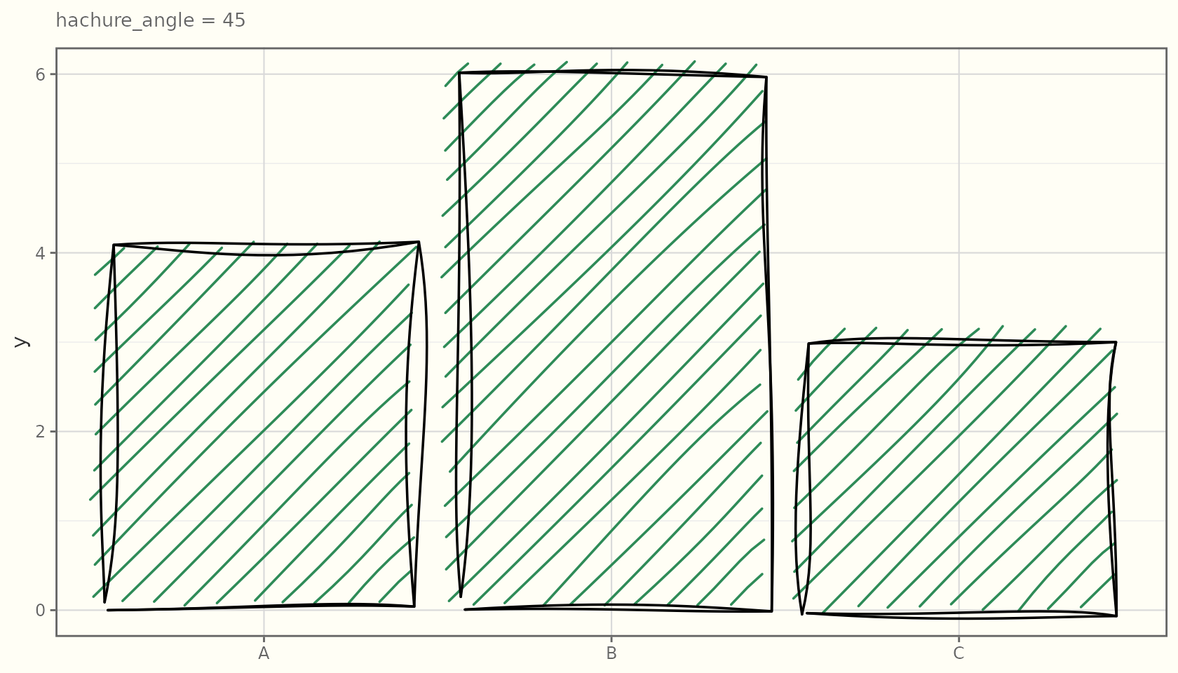
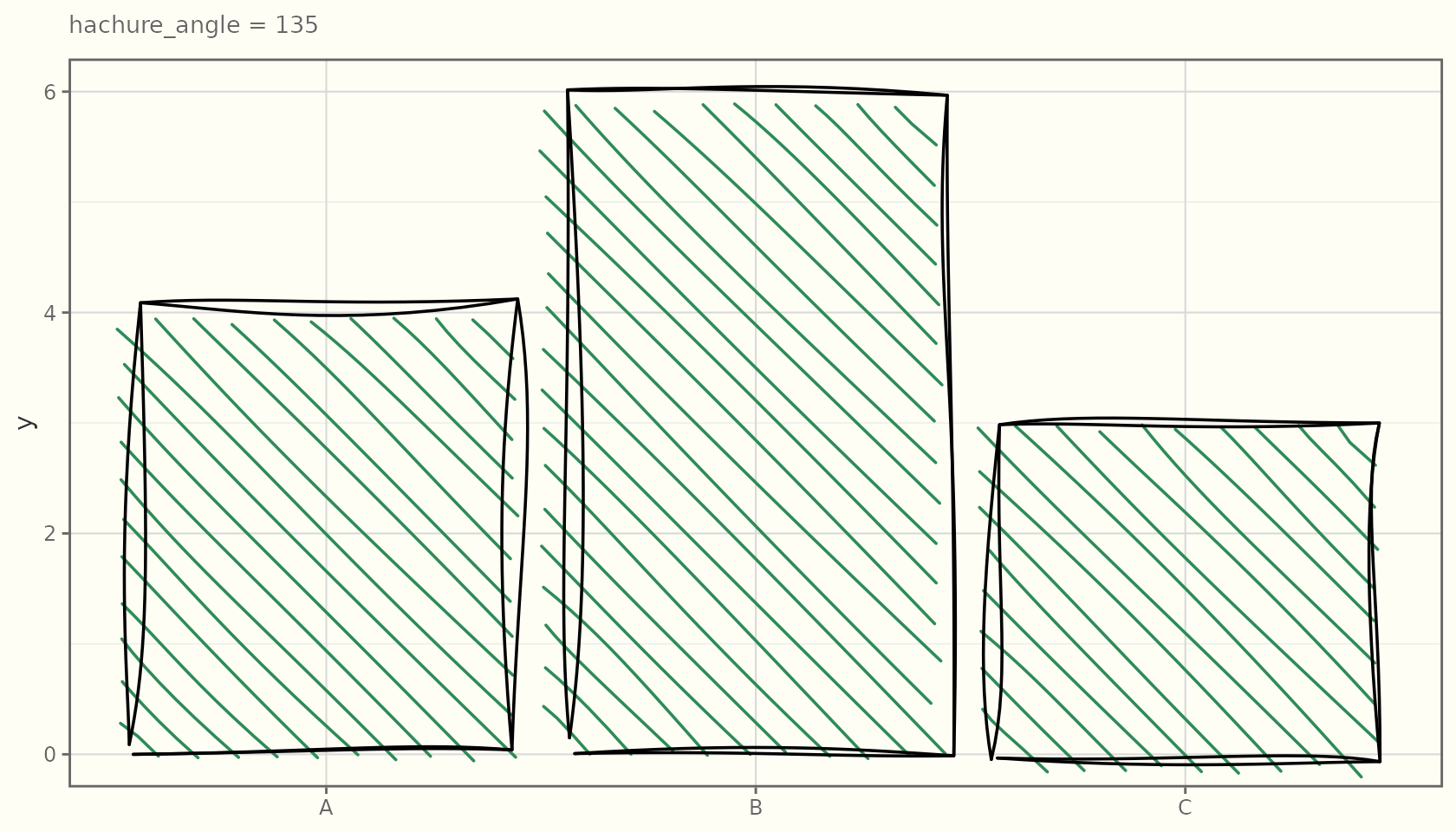
hachure_angle

The angle (degrees) of the fill lines:

df <- data.frame(x = c("A", "B", "C"), y = c(4, 6, 3))
for (a in c(0, 45, 90, 135)) {
  print(
    ggplot(df, aes(x, y)) +
      geom_sketch_col(fill = "seagreen", hachure_angle = a, seed = 1L) +
      labs(subtitle = paste("hachure_angle =", a), x = NULL) +
      theme_sketch(base_size = 9)
  )
}

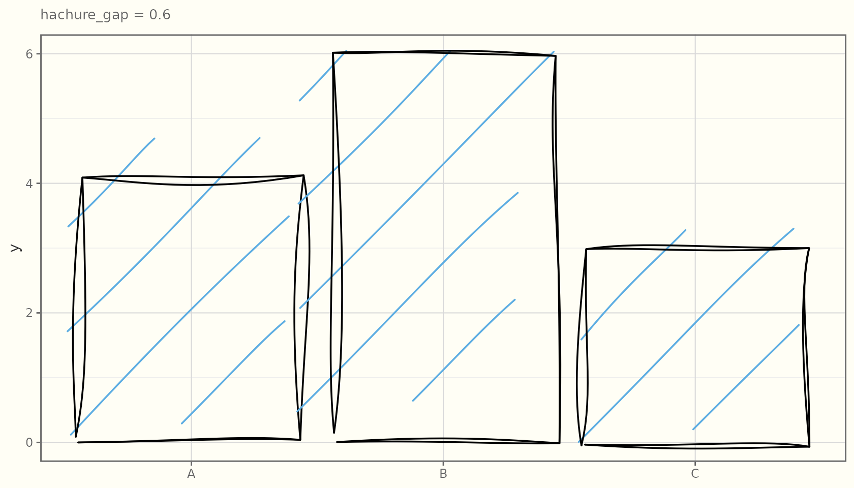
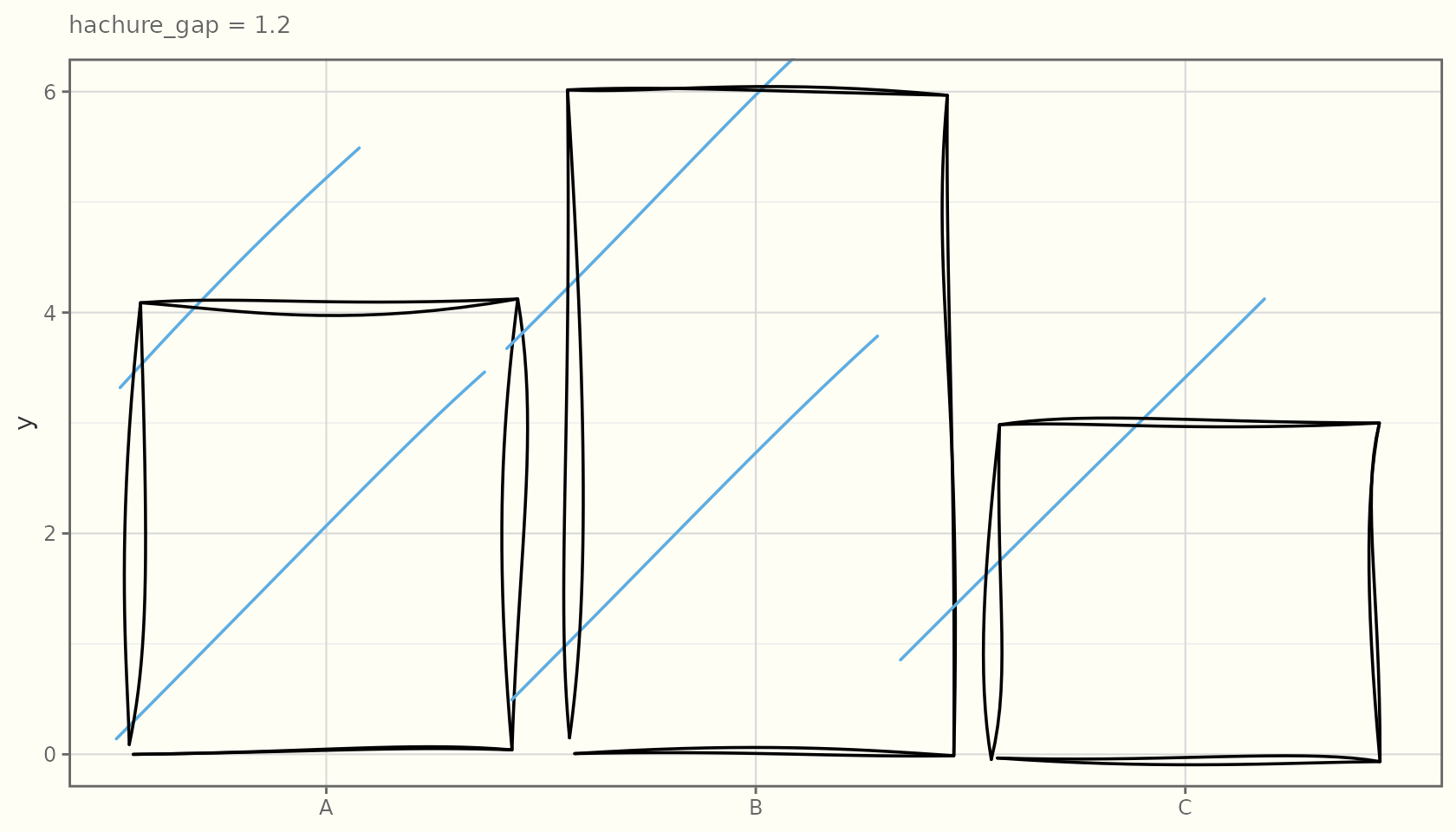
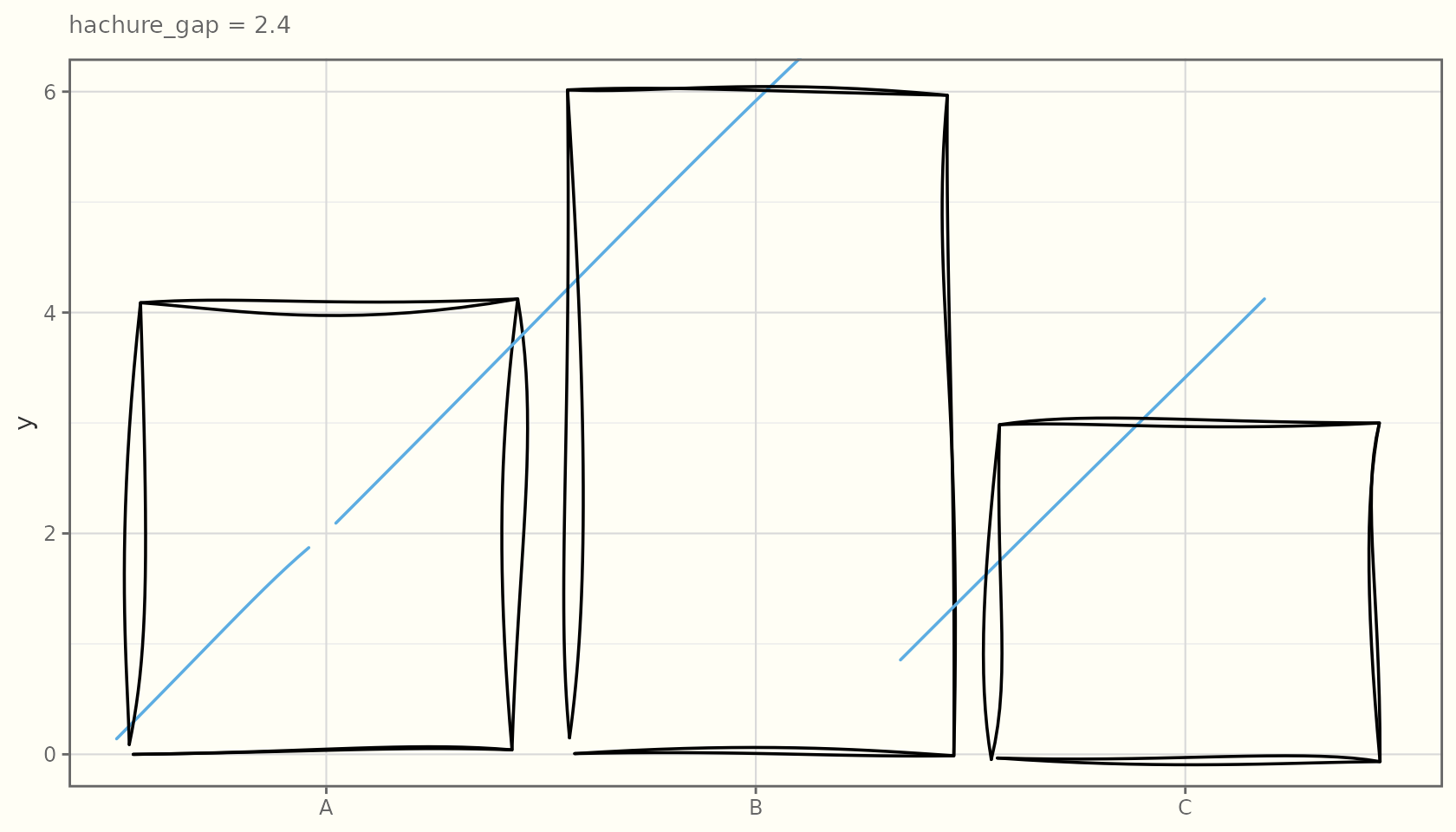
hachure_gap

Spacing between fill lines, in data units — smaller means denser shading:

for (g in c(0.6, 1.2, 2.4)) {
  print(
    ggplot(df, aes(x, y)) +
      geom_sketch_col(fill = "#5DADE2", hachure_gap = g, seed = 1L) +
      labs(subtitle = paste("hachure_gap =", g), x = NULL) +
      theme_sketch(base_size = 9)
  )
}

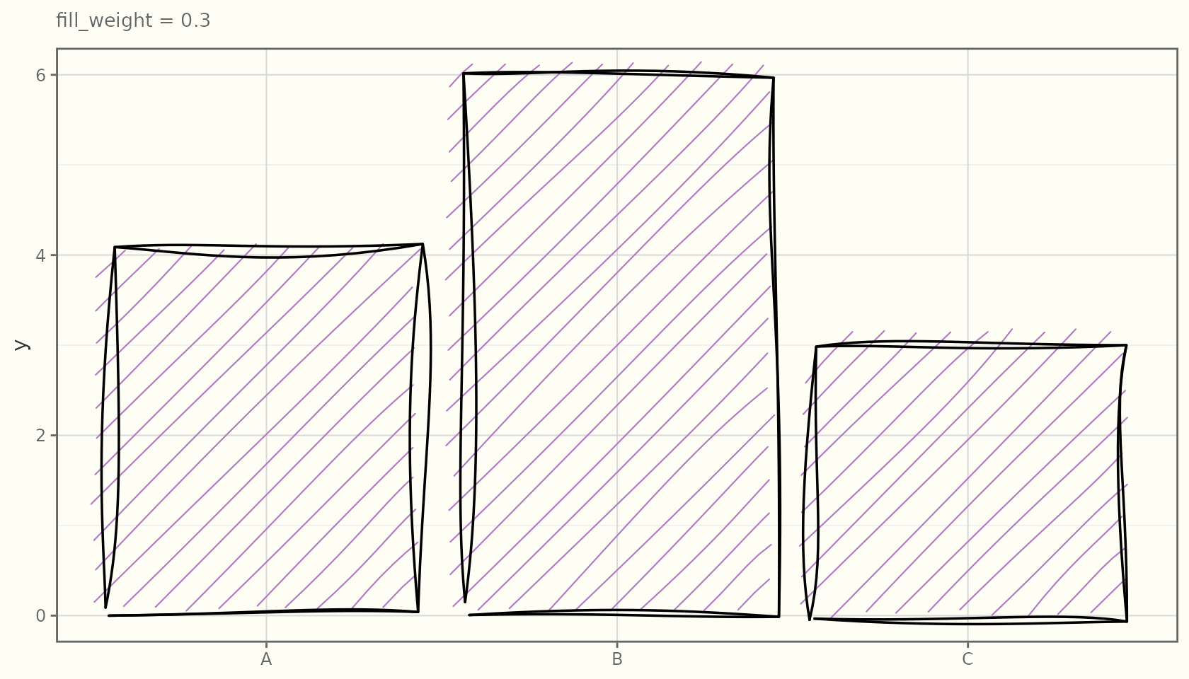
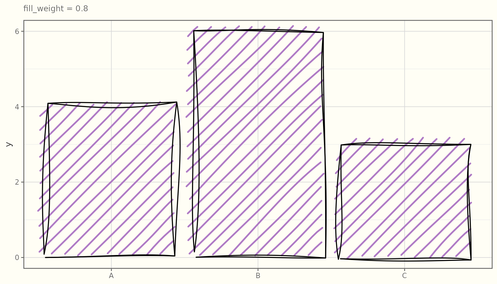
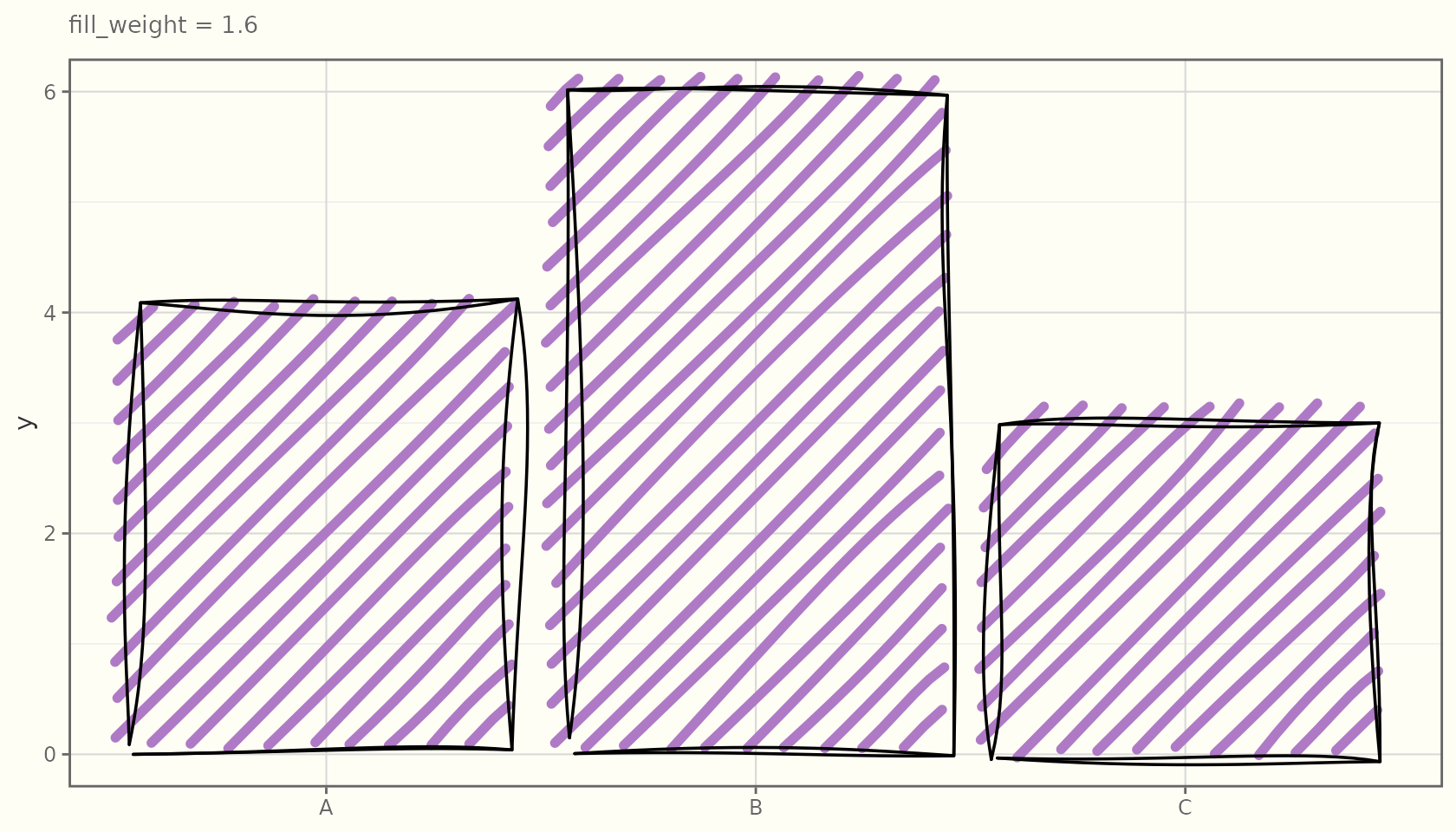
fill_weight

The stroke weight of the fill lines:

for (w in c(0.3, 0.8, 1.6)) {
  print(
    ggplot(df, aes(x, y)) +
      geom_sketch_col(fill = "#AF7AC5", fill_weight = w, seed = 1L) +
      labs(subtitle = paste("fill_weight =", w), x = NULL) +
      theme_sketch(base_size = 9)
  )
}

Fills follow the shape

Because the filler is a true scan-line algorithm, the texture conforms to any polygon outline, not just rectangles:

ang  <- seq(0, 2 * pi, length.out = 9)[-9]
hex  <- data.frame(x = cos(ang), y = sin(ang))
ggplot(hex, aes(x, y)) +
  geom_sketch_polygon(fill = "#E74C3C", fill_style = "cross_hatch",
                      hachure_angle = 30, seed = 1L) +
  coord_equal() +
  labs(title = "Cross-hatch on a hexagon") +
  theme_sketch()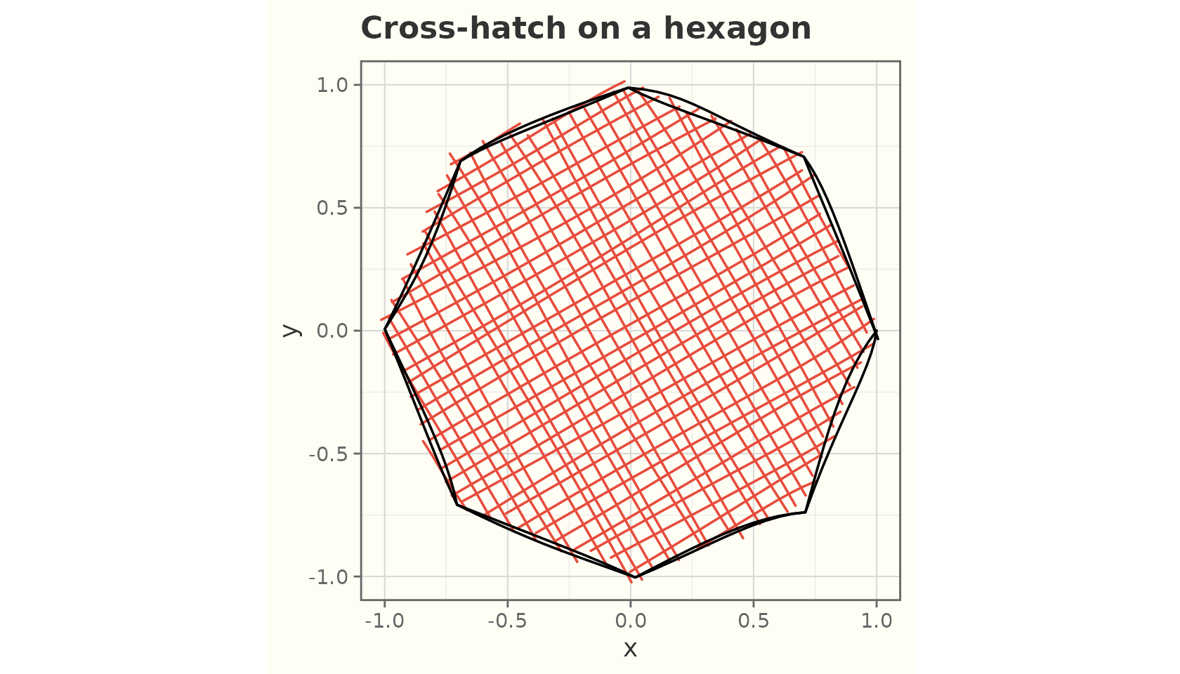

td <- expand.grid(x = 1:5, y = 1:3)
td$z <- td$x
ggplot(td, aes(x, y, fill = z)) +
  geom_sketch_tile(fill_style = "dots", seed = 1L) +
  scale_fill_viridis_c() +
  labs(title = "Dotted tiles") +
  theme_sketch()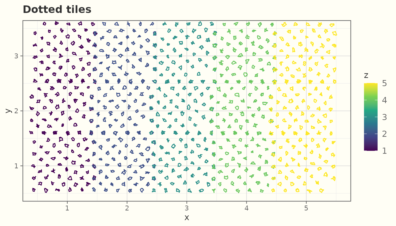

Working directly with the filler

The fill geometry comes from pure Layer-1 functions you can call yourself — useful for testing or custom grobs. sketch_fill() dispatches to the styles and returns a list of line segments:

square_x <- c(0, 1, 1, 0)
square_y <- c(0, 0, 1, 1)
segs <- sketch_fill(square_x, square_y, fill_style = "hachure",
                    hachure_gap = 0.15, seed = 1L)
length(segs)      # number of fill segments
#> [1] 8
head(segs[[1]])   # each segment is a matrix of x/y points
#>              x          y
#> [1,] 0.7093499 0.07633409
#> [2,] 0.8440814 0.20310311
#> [3,] 0.9270041 0.27937282