Continuous scale for the engraving tone aesthetic

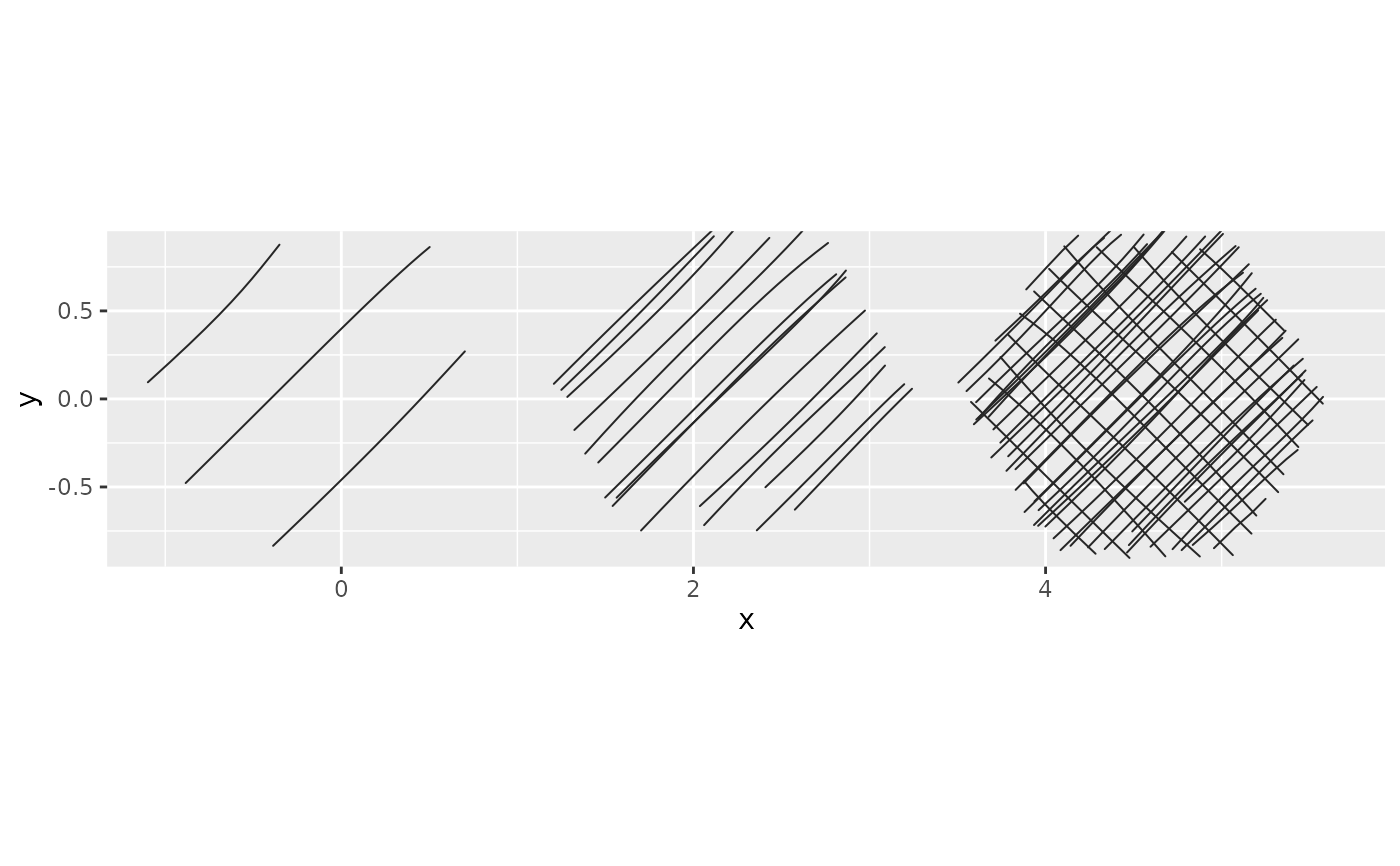
geom_sketch_shade() shades each region by a tone aesthetic in [0, 1] (0 = blank paper, 1 = densest cross-hatch). Mapping a raw variable to tone (aes(tone = z)) rescales its observed range to a legible tone band with this scale, just as scale_size() rescales to a size range. It is applied automatically whenever tone is mapped to a continuous variable, so you only call it directly to change range (or to reverse it by giving a decreasing range). To use values as raw tone with no rescaling, wrap them in base::I() (aes(tone = I(z))).

Usage

scale_tone_continuous(..., range = c(0.15, 0.95), guide = "none")

scale_engrave(..., range = c(0.15, 0.95), guide = "none")

Arguments

...

Other arguments passed to ggplot2::continuous_scale().

range

Output tone range, within [0, 1]. Default c(0.15, 0.95): 0.15 is the faintest hatch that still draws (the engraving ladder leaves tone below 0.12 as blank paper, so a lower floor would erase the lightest region entirely) and 0.95 is near-solid black. Give a decreasing range (e.g. c(0.95, 0.15)) to invert the mapping.

guide

Legend guide. Defaults to "none" because the legend keys do not reflect tone; set to "legend" to show one anyway.

Value

A ggplot2 scale object.

See also

Other sketch-theme: CoordSketch, CoordSketchPolar, element_sketch_line(), ggsketch_check_fonts(), ggsketch_save(), register_sketch_font(), scale_pressure_continuous(), scale_roughness_continuous(), scale_sketch, sketch_palette(), theme_sketch()

Examples

library(ggplot2)

hex <- data.frame(
  x = cos(seq(0, 2 * pi, length.out = 7))[-7],
  y = sin(seq(0, 2 * pi, length.out = 7))[-7]
)
regions <- do.call(rbind, lapply(1:3, function(k) {
  transform(hex, x = x + (k - 1) * 2.3, g = k, val = k)
}))

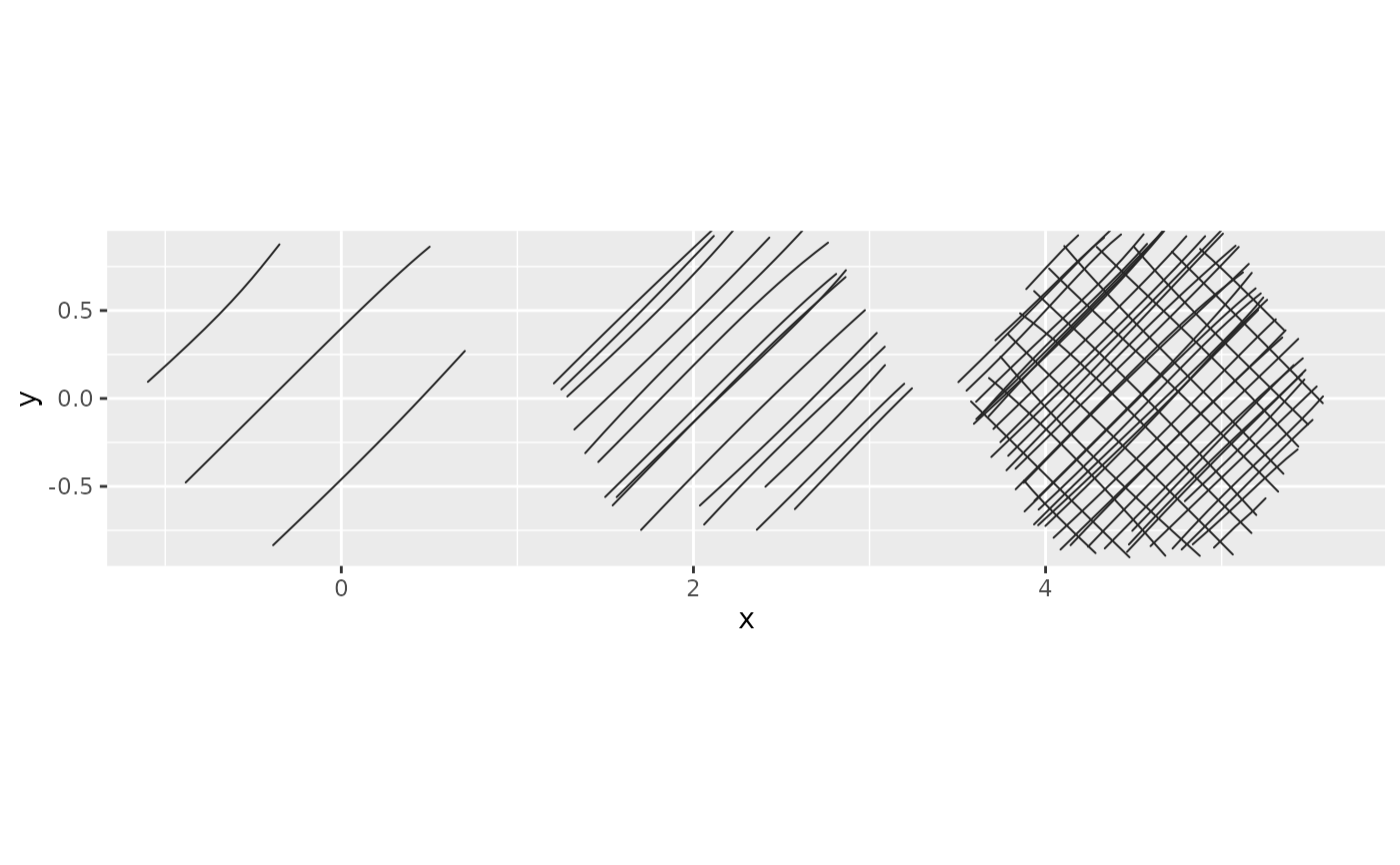
# `val` is rescaled to the default tone band c(0.15, 0.95) automatically.
ggplot(regions, aes(x, y, group = g)) +
  geom_sketch_shade(aes(tone = val), seed = 1L) +
  coord_equal()


# Push the darkest region all the way to solid black.
ggplot(regions, aes(x, y, group = g)) +
  geom_sketch_shade(aes(tone = val), seed = 1L) +
  scale_tone_continuous(range = c(0.15, 1)) +
  coord_equal()